How to Create a Combo Chart in Microsoft Excel

When you want to display different data sets visually, you can create a combination chart. If you want to show something like sales with costs or traffic with conversions, a combo chart in Microsoft Excel is ideal.

We’ll show you how to create a combo chart in Excel as well as customize it to include the elements you need and give it an attractive appearance.

Table of Contents

How to Create a Combo Chart in Excel

You have a few ways to create a combo chart in Excel. You can convert an existing chart, select a quick combo chart type, or set up a custom chart.

Convert an Existing Chart to a Combo Chart

If you already have a chart showing your data, like a bar chart or even a pie chart, you don’t have to delete it and start from scratch. Simply turn it into a combo chart.

Select your current chart and go to the Chart Design tab.
Choose Change Chart Type in the Type section of the ribbon.

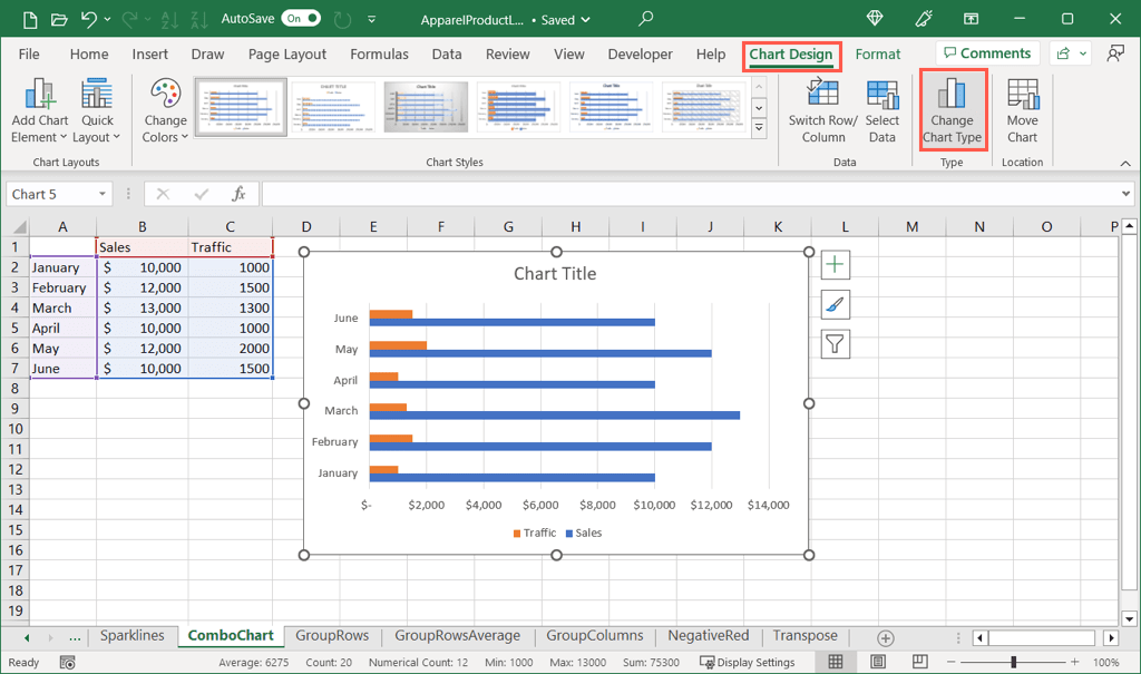
When the chart window opens, pick Combo on the left.
Then, select one of the combo chart layouts at the top and customize the series at the bottom.

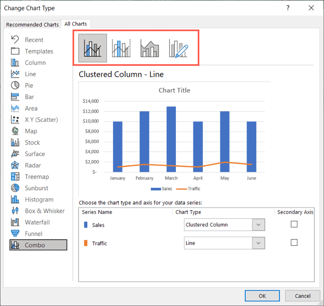
Choose OK and you’ll see your new chart replace the original one.

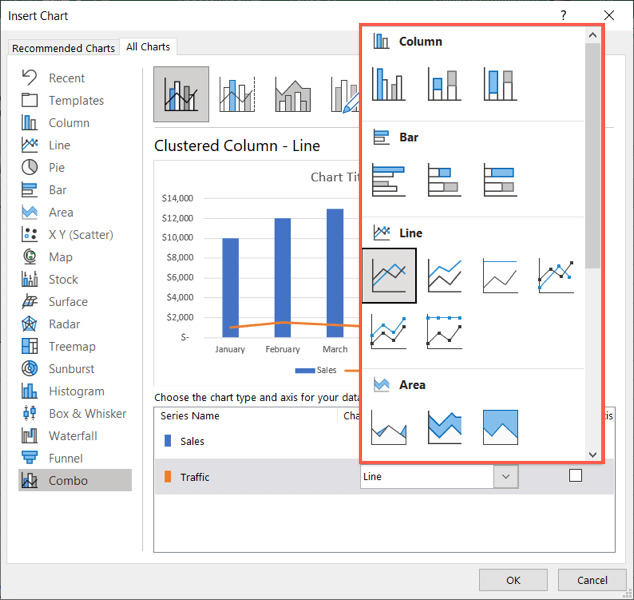
Select a Quick Combo Chart Type

Excel offers three combo chart types that you can pick from for your data.

Select your data set and go to the Insert tab.

In the Charts group, choose the Insert Combo Chart drop-down arrow to see the options. Pick from a clustered column with a line chart, a clustered column and line chart with a secondary axis, or a stacked area and clustered column chart.

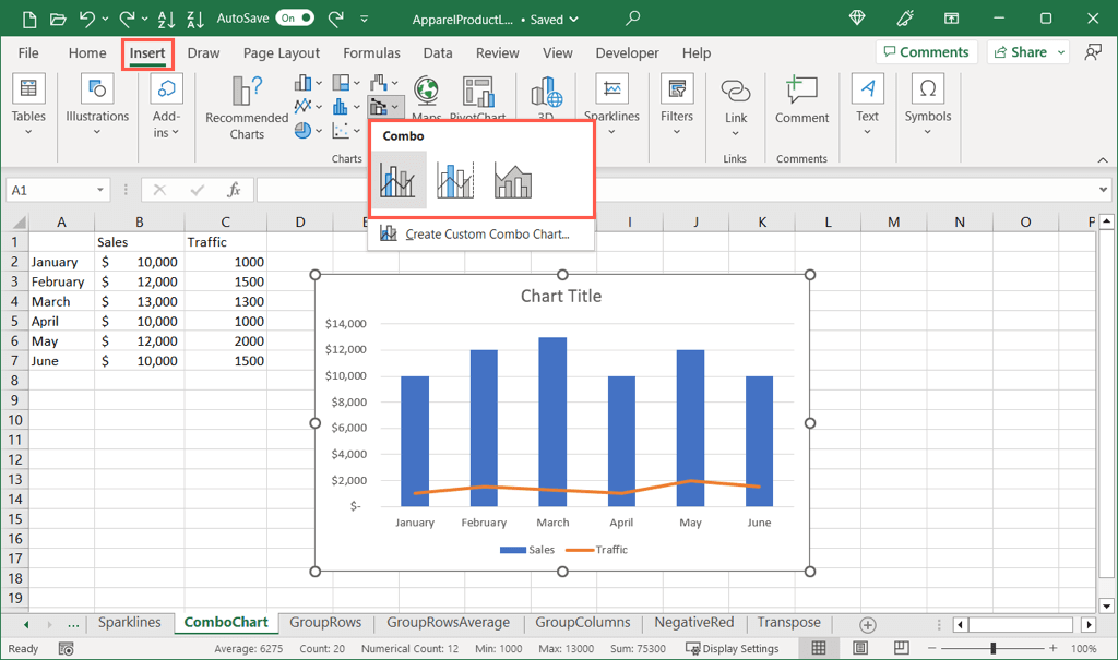
You’ll then see the chart type you pick pop right onto your spreadsheet.

Create a Custom Combo Chart

If you don’t have an existing chart and prefer to customize the series and axis for the combo chart from the start, you can create a custom chart.

Select your data set and go to the Insert tab.
Choose the Insert Combo Chart drop-down arrow and pick Create Custom Combo Chart.

When the chart window opens, you’ll see four combo chart types at the top. Select one of these as the base for your custom chart.

At the bottom, you’ll see your data series, chart types, and options to pick a secondary axis. As you make your adjustments, you’ll see a nice preview of the combo chart directly above.

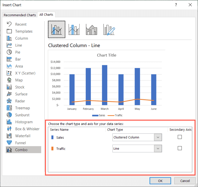
While a column chart and line graph work well together, you can choose a different chart type for each data series if you like. Select the drop-down box below Chart Type to the right of the series you want to change and select the new chart type.

By default, the first data series displays on the primary axis. However, you can change this or simply add a secondary axis using the Secondary Axis check boxes on the right side.

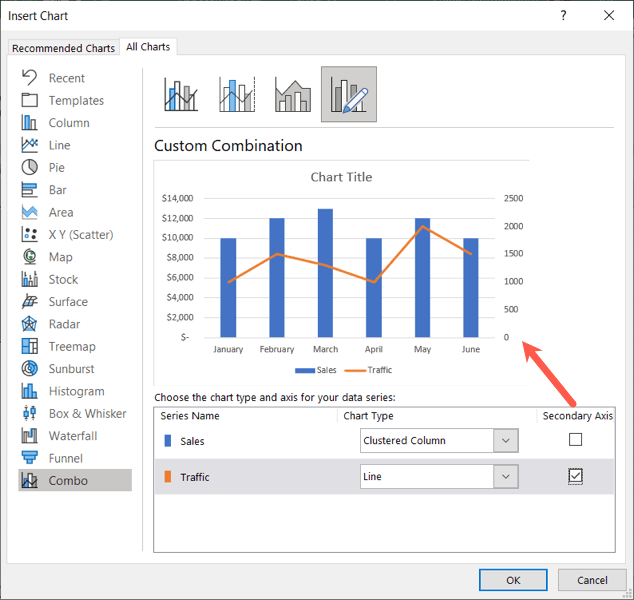
When you finish creating your custom combo chart, pick OK to save it and place it on your worksheet.

How to Customize a Combo Chart

Once you choose and insert your combo chart, you may want to add more elements or give the chart some pizzazz. Excel offers several features for customizing a chart.

Go to the Chart Design Tab

For basic appearance features and chart elements, select your chart and go to the Chart Design tab.

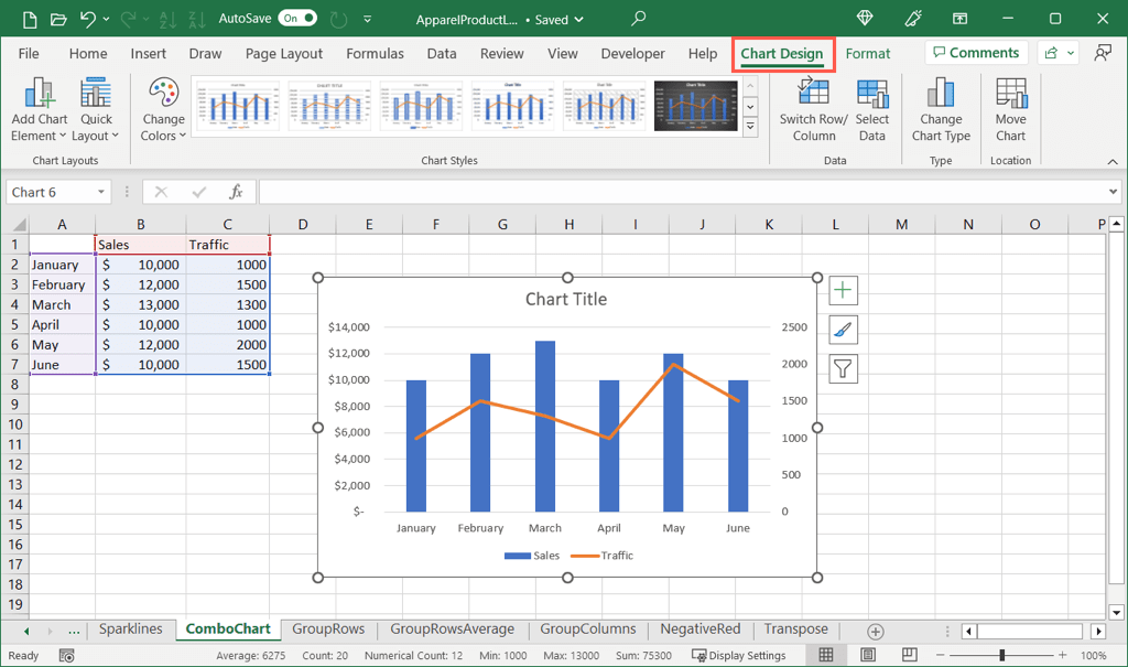
Starting on the left side of the ribbon, you can use the Add Chart Element drop-down menu to add and position items like the chart title, data labels, and legend.

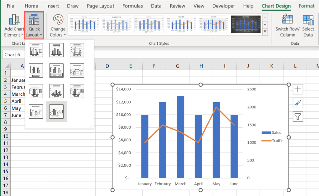
To the right, use the Quick Layout menu to change the layout to include and position elements without having to do so one-by-one.

In the Chart Styles section, you can use the Change Colors drop-down menu to pick a different color scheme or the Styles box to choose a whole new design.

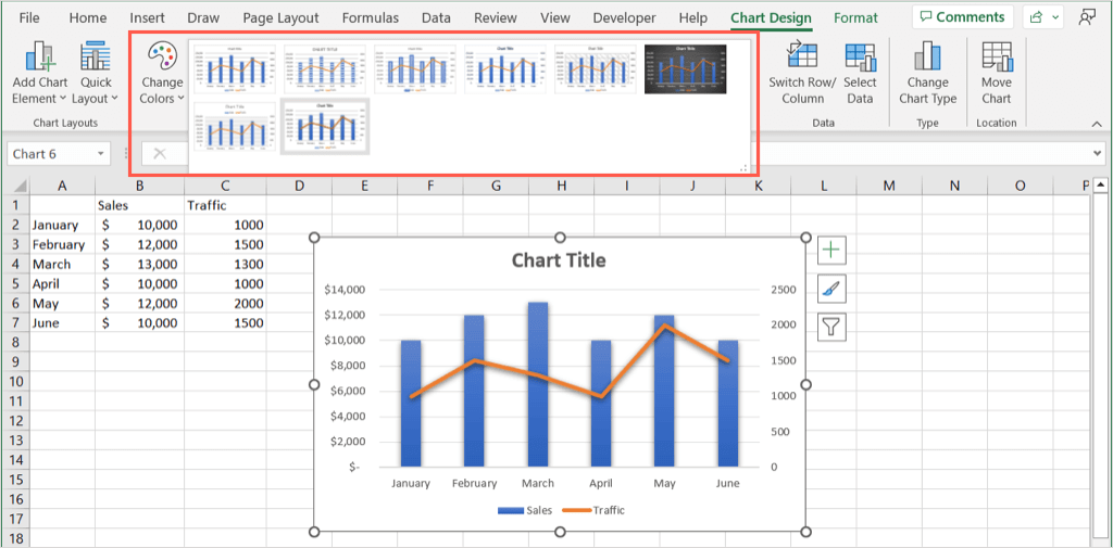
With the remaining options on the ribbon, you can switch columns and rows, change the chart data selection, pick a new chart type, or move the chart to another sheet.

Open the Format Chart Area Sidebar

For changing the chart font, adding a border, and positioning the chart and text, right-click the chart and choose Format Chart Area. This opens a sidebar on the right where you can make more detailed adjustments.

Use Chart Options or Text Options at the top of the sidebar depending on which item you want to change. You can then use the tabs directly beneath to make your changes.

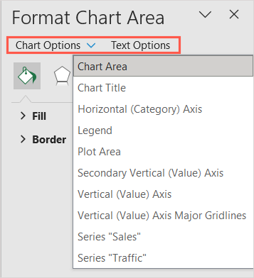
Chart Options: Change the fill and border styles and colors, add effects like a shadow or soft edge, and set the size or position for the chart.

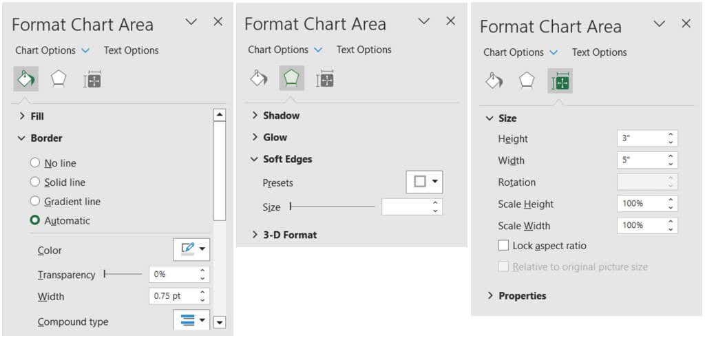
Text Options: Change the fill or outline styles and colors, add effects, and position or align the text.

Use the Chart Buttons (Windows Only)

One more way to make adjustments to your chart is to use the buttons that display on the right side of it. These are currently only available in Microsoft Excel on Windows, not Mac.

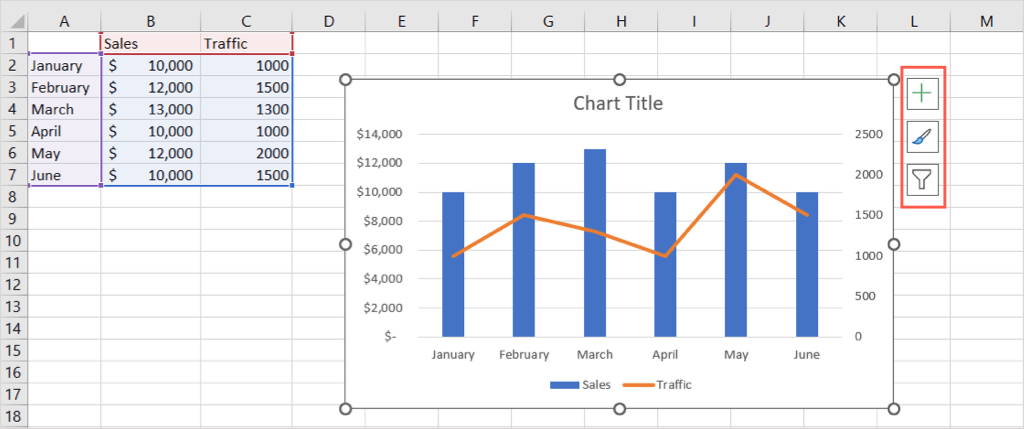
Chart Elements (plus sign): Like the Chart Elements drop-down box on the Chart Design tab, you can add, remove, and position items on the chart.

Chart Style (paint brush): Like the Chart Styles section on the Chart Design tab, you can pick a different color scheme or style for your chart.

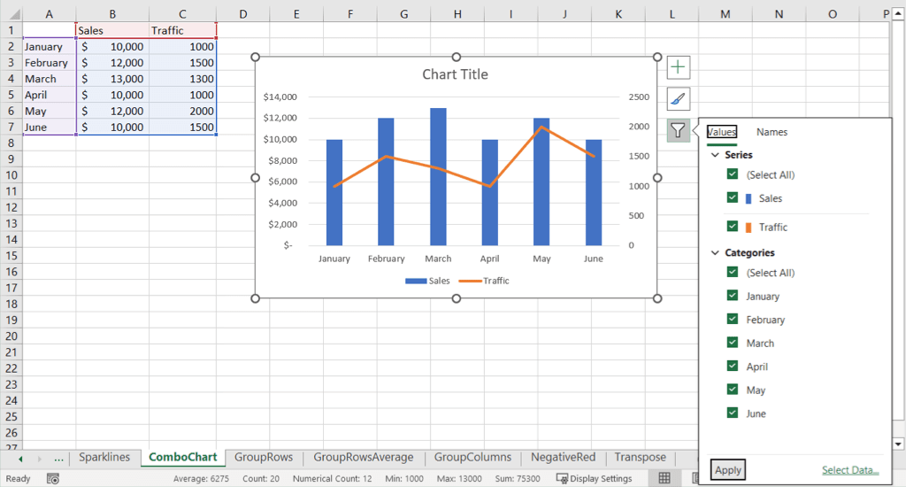
Chart Filters (filter): With this button, you can check or uncheck the details in your dataset that you want to display on your chart. This gives you a quick way to view only specific chart data by hiding other details temporarily.